Options Risk Profiles

Options risk profiles provide a visual and quantitative map of how an option position gains or loses value under different market conditions. They serve as the backbone of structured options trading because they translate contract terms into a clear statement of potential outcomes. A risk profile is not a prediction. It is a conditional statement about what would happen to profit and loss if price, volatility, and time move in specific ways. When used consistently, risk profiles help traders standardize decision rules, evaluate trade-offs, and monitor risks with greater discipline.

What Is an Options Risk Profile

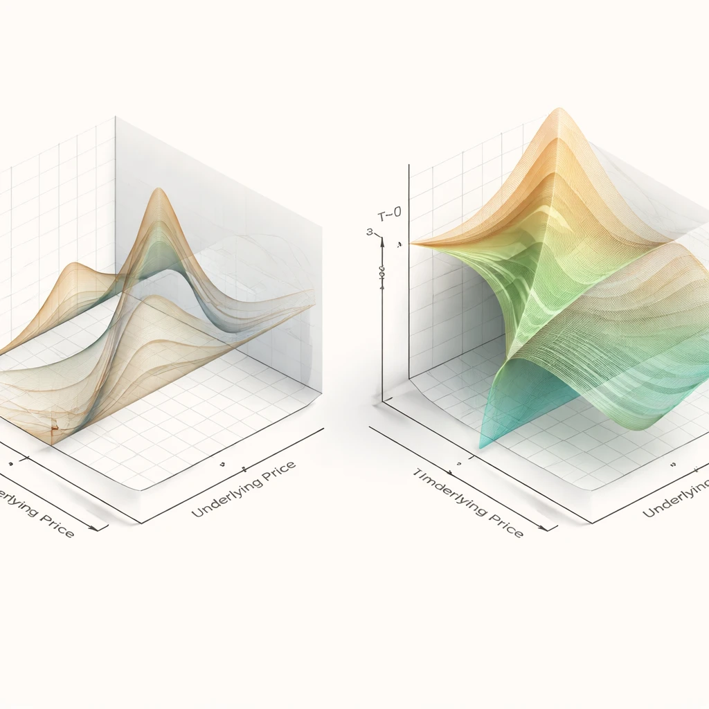
An options risk profile is a representation of a position’s expected profit or loss across a range of underlying prices, times to expiration, and implied volatility levels. The most common representation is a two-dimensional payoff diagram at expiration that shows cumulative profit or loss versus the underlying’s price on expiration day. A more informative representation adds non-expiration curves, sometimes called T-0 or T-n profiles, which incorporate time value and implied volatility. The full concept is three-dimensional because profit and loss depend simultaneously on price, volatility, and time.

Risk profiles are constructed from the position’s contracts, including strike prices, option type, quantity, side, and expiration dates. The option pricing model, whether Black-Scholes-Merton or a more advanced volatility surface model, maps these inputs to current option values and sensitivities. From these components, the profile reveals how the position responds to scenarios such as a 5 percent price increase, a 10 percent volatility shock, or a week of time decay.

Core Logic Behind Risk Profile Construction

At expiration, option values reduce to intrinsic value. A long call is worth max(S - K, 0). A long put is worth max(K - S, 0). Combinations add these pieces linearly. The expiration diagram for any multi-leg position is the sum of the piecewise linear payoffs of its legs. This creates the characteristic shapes associated with spreads, straddles, strangles, butterflies, condors, covered calls, and protective puts.

Before expiration, profiles include extrinsic value, which reflects time to expiration and implied volatility. The non-expiration curve is therefore smoother and usually less extreme than the expiration line. The gap between these curves is the value of optionality. It shrinks as time passes and as volatility falls, and it grows as volatility rises. Traders often analyze both the expiration profile and one or more pre-expiration profiles to understand how the position evolves.

Greeks translate the shape of the profile into local sensitivities. Delta is the slope of the profile with respect to price. Gamma measures how quickly delta changes with price, which affects the curvature of the profile. Theta measures the effect of time passing, often negative for long premium positions and positive for short premium structures. Vega measures sensitivity to implied volatility changes, which shifts the profile up or down for long vega positions and in the opposite direction for short vega positions. Rho captures rate sensitivity for longer-dated options. While the full risk profile is global and scenario-based, the Greeks provide a local description around current market conditions that helps with monitoring and adjustment.

Reading Payoff Shapes

Interpreting a risk profile requires linking the visual shape to the underlying economic exposure. Consider several canonical examples to illustrate the logic. These are not recommendations. They are archetypes used to explain how the shapes encode risk and reward.

• Long call: Limited downside to the premium paid, uncapped upside as the underlying rises. Positive delta, positive gamma, negative theta, positive vega. The profile steepens on rallies and flattens on declines.
• Long put: Limited downside to the premium, gains if the underlying falls. Negative delta, positive gamma, negative theta, positive vega.
• Vertical spread: Limited risk and limited reward. A bull call spread gains if price rises within a range, with capped upside. A bear put spread gains if price falls within a range, with capped downside protection. The profile smooths out extremes relative to a single option.
• Straddle or strangle: Seeks movement regardless of direction. Gains from large moves up or down. Strongly negative theta, strongly positive vega, high gamma near the strikes.
• Iron condor or iron butterfly: Gains if price remains within a range, loses if it breaks through the short strikes. Typically positive theta and negative vega. Risk is concentrated around the wings and can change quickly as price approaches short strikes.
• Calendar spread: Long farther-dated option and short nearer-dated option with the same strike. Positive vega exposure and a localized profit region around the strike. Sensitive to the evolution of the volatility term structure.

Each shape embeds assumptions about likely price paths, volatility behavior, and time horizons. Structured trading systems rely on aligning these shapes with defined market regimes and with the trader’s capital constraints.

Expiration Profiles Versus Live Risk

It is common to focus on the expiration diagram because it is intuitive and piecewise linear, but live risk is determined by the pre-expiration profile. A position with apparent limited risk at expiration can experience significant interim losses if volatility rises or if price moves rapidly toward a risk boundary. Short option structures highlight this distinction. A short vertical spread has capped risk at expiration, yet mark-to-market losses can climb early if the underlying accelerates toward the short strike with a volatility jump.

Therefore, risk profiles should be examined across multiple time slices. A practical workflow is to inspect the T-0 curve, the profile one week forward, and the expiration line. This shows how time decay and potential volatility changes alter the position’s cushion and risk points.

Risk Management Considerations

Risk profiles are most valuable when they inform concrete risk controls inside a system. The following categories are commonly codified in trading rules. None are prescriptive, but each highlights how the profile translates into operational safeguards.

• Defined risk versus undefined risk: Structures with capped loss at expiration, such as long options and debit spreads, present different monitoring needs than short options and credit spreads with potentially larger interim swings. The profile makes this distinction explicit.
• Concentration and correlation: Summed profiles across positions can create unintended clusters of risk around certain price regions. Aggregating profiles within the same underlying and across correlated underlyings helps identify crowded exposures.
• Volatility regime sensitivity: Positions with negative vega, such as short premium structures, can appear stable until implied volatility rises. Scenario testing the profile under volatility shocks provides a clearer view of drawdown potential.
• Liquidity and assignment risk: American-style options on single stocks can be exercised early. Profiles should be evaluated with the operational possibility of early assignment, especially around dividends or deep in-the-money short options.
• Margin and capital utilization: Brokers compute margin based on a model of the position’s risk. The live profile should be reconciled with margin requirements to avoid forced reductions if volatility jumps or if price approaches risk boundaries.
• Adjustment thresholds: Some systems define pre-set points at which the shape becomes inconsistent with the strategy’s goals, such as delta limits or proximity to short strikes. The risk profile provides the basis for where those triggers sit.
• Event risk: Earnings, macro releases, and ex-dividend dates can change implied volatility and gap risk. Profiles can be stress-tested around such events to evaluate whether the shape remains acceptable.

Building Risk Profiles Into a Structured Trading System

A structured system starts with a hypothesis about market conditions and selects a risk profile that matches that hypothesis. The process is repeatable when the mapping from conditions to profiles is explicit, measurable, and consistently applied. The core components can be organized as follows.

• Regime definition: Specify observable features such as trend filters, realized volatility states, skew levels, or earnings calendar status. The objective is to define when a given payoff shape is appropriate.
• Profile selection: Choose a position structure whose expiration and pre-expiration profiles align with the regime. For example, a narrow profit zone favored by a range-bound regime will differ from a convex profile preferred in a high-uncertainty regime.
• Risk limits: Translate the profile into maximum acceptable drawdowns under scenario tests, margin usage caps, delta or vega limits, and concentration rules across strikes and symbols.
• Position sizing logic: Base size on profile-defined risk rather than premium collected or paid. The relevant metric could be the worst-case scenario under a defined shock, or a margin-based constraint consistent with historical stress.
• Monitoring and adjustments: Use the Greeks and the evolving T-0 profile to decide when the position has drifted from its intended shape. Adjustments can change strikes, add hedges, or reduce exposure, depending on the framework.
• Exit and review: Exit conditions can be time-based, profile-based, or event-based. After closure, compare realized path-dependent P and L with the scenarios that informed the initial choice.

Scenario Analysis and Stress Testing

Scenario analysis is the engine behind risk profile evaluation. The minimum useful set spans discrete moves in the underlying price, parallel and non-parallel changes in implied volatility, and time steps. A common grid might include price moves of fixed percentage increments, volatility shocks of several points up or down, and time advances that reflect realistic holding periods. The output is a matrix of potential profit or loss values, which can be summarized by quantiles or worst-case outcomes within reasonable bounds.

Stress tests extend beyond the typical grid to include gaps, skew changes, and cross-gamma effects in multi-leg positions. For example, an iron condor’s short options may localize risk near the short strikes, but skew steepening during a selloff can increase the losses relative to a parallel volatility shock. A calendar spread may react differently to a front-month volatility spike than to a back-month spike. Stress testing aims to capture these second-order effects that the simpler expiration diagram cannot reveal.

Greeks as Live Risk Diagnostics

While the profile shows outcomes over ranges, the Greeks summarize the near-term risk around current conditions. Systems often set guardrails using Greek exposures.

• Delta: Indicates directional exposure. Position-level delta limits help keep overall direction contained even if individual strategies have tilt.
• Gamma: Signals how quickly delta can change. Short gamma can mean losses accelerate on large moves, which is often paired with positive theta. This trade-off is a central feature of many short premium profiles.
• Theta: Measures time decay. Positive theta positions may benefit from passing time in quiet markets, while negative theta profiles rely on movement to offset decay.
• Vega: Captures sensitivity to volatility changes. Negative vega structures can face losses when markets reprice uncertainty higher.
• Cross-Greeks: Higher-order terms like vanna and volga can matter for multi-leg and longer-dated positions because they affect how the profile shifts when volatility and price move together.

Diagnostics are useful when tied to actions defined by the system. For instance, a system may constrain portfolio-level net delta within a band and reduce exposure if gamma risk rises beyond a threshold prior to an event. These are process choices, not predictions.

Path Dependency and Early Exercise

Options are path dependent because time, volatility, and price do not move in straight lines. A position’s interim drawdowns can differ widely from its expiration outcomes. Risk profiles should be interpreted with that path dependency in mind. Early exercise of American-style options introduces additional paths. Short in-the-money calls ahead of ex-dividend dates, for example, may be exercised early when extrinsic value is small relative to the dividend. A system that relies on holding to expiration must incorporate operational steps for managing assignment risk. Profiles are built on valuation models, but live management must reconcile model assumptions with market microstructure and contract features.

Volatility Surfaces and Skew

Real markets price volatility differently across strikes and maturities. Skew and term structure are not incidental. They shape the risk profile, especially for multi-leg positions. For instance, an out-of-the-money put often carries higher implied volatility than an equidistant call. That affects the cost of downside protection and the reward of selling downside premium. A spread built with options at different relative moneyness levels inherits those skews. Calendar spreads are sensitive to the slope and curvature of the term structure, not only the level of volatility. Scenario analysis that holds volatility constant may misstate risks if skew or term changes are likely under the contemplated regime.

Time and Decay Dynamics

The pace of time decay accelerates as expiration approaches, all else equal. The result is a profile whose non-expiration curve converges toward the expiration line more rapidly in the final days. For long premium positions, this acceleration creates a steeper hurdle for realized movement to overcome. For short premium structures, the same dynamic can shrink risk if price stays within a favorable range, but it can also reduce maneuvering time if price drifts toward a boundary late in the cycle. Systems that rely on narrow profit zones often incorporate time-based exits or roll logic that is consistent with the way theta accelerates.

Margin, Capital, and Portfolio Aggregation

Margin models across brokers differ, but they share the goal of quantifying potential losses. Portfolio margin frameworks approximate risk using scenario-driven assumptions. Standard margin rules apply fixed formulas tied to position types. In both cases, the live risk profile should be reconciled with the margin method to avoid procyclical constraints. When implied volatility rises, margins typically increase, sometimes sharply. A conservative system designs position sizes that remain manageable under plausible margin expansions.

Aggregation is critical. A single position might appear modest in isolation, but a portfolio of similar structures across correlated equities can concentrate risk in a single price range or volatility outcome. Summing position-level profiles into a portfolio-level profile helps reveal overlapping exposures. This can be done per underlying, sector, or factor, and is often more informative than monitoring only Greeks at the position level.

Data and Tooling Requirements

Consistent use of risk profiles in a system requires reliable data and tools. Historical price series, implied volatility surfaces, corporate action calendars, and event schedules form the data backbone. The tooling should support multi-slice profiles, scenario matrices, and aggregation across positions. The ability to export scenario results, archive them with the trade record, and compare them with realized outcomes improves feedback for system refinement. Model risk is real. Using multiple models or performing sensitivity checks on key inputs can reduce overconfidence in any single valuation approach.

High-Level Operating Example

Consider a system designed to deploy range-bound profiles during stable volatility regimes and convex profiles during uncertain regimes. The following sequence illustrates the role of risk profiles without specifying entries or exits.

• Regime identification: The system classifies the current environment as range-bound based on realized volatility within predefined bands and the absence of near-term idiosyncratic events. Implied volatility is near its 3-month median.
• Profile selection: The system selects a limited-risk, income-oriented structure with a profit zone centered around the prevailing price level. The expiration profile shows a plateau of potential profit if price stays within the zone, with capped losses defined by long wings. The T-0 curve is shallower than expiration but aligned with the intended range.
• Scenario test: The profile is evaluated under price moves of several increments in both directions, with volatility shocks up and down, and a time step consistent with the planned holding period. The system records the worst-case loss within this grid and confirms it is within risk limits.
• Sizing and concentration controls: Position size is set so that the worst-case loss from the scenario grid fits within a fixed percentage of allocated capital, while aggregate portfolio delta and vega remain inside limits.
• Monitoring: As days pass, the T-0 curve shifts. If price drifts toward the short strike region and the system’s delta limit is breached, an adjustment is considered. If implied volatility rises beyond a threshold, the system re-runs the scenario grid to check whether drawdowns remain within bounds.
• Exit and review: On exit, realized P and L and path are compared with the scenario matrix. If realized drawdown exceeded expectations despite staying inside the price range, the system reviews assumptions about skew or term structure changes that may have altered the profile.

This example shows how the risk profile acts as a decision anchor at each stage, from selection to monitoring to review, without relying on discretionary interpretation.

Common Misinterpretations

Several pitfalls recur when traders rely on partial views of the profile.

• Confusing expiration diagrams with live P and L: The expiration line is not the position’s current risk. Non-expiration curves and scenario analysis are necessary for realistic expectations.
• Ignoring volatility skew dynamics: Assuming parallel volatility shifts can misstate risk. Skew and term structure often change in asymmetric ways during market stress.
• Overreliance on single-number metrics: A position’s theta or delta is incomplete without context. The full profile and scenario grid are required to understand how those metrics evolve with movement.
• Neglecting assignment mechanisms: Early exercise risk is operational and can alter the profile abruptly. Systems should anticipate these events.
• Underestimating aggregation effects: Summed exposures across positions can create sharp portfolio-level cliffs that are not visible at the trade level.

Documentation and Repeatability

Structured systems benefit from documentation that makes the link between market conditions and chosen profiles explicit. A concise checklist can support this goal.

• Define the intended regime and its observable indicators.
• Record the targeted payoff shape and its rationale.
• Store the scenario matrix results, including price, volatility, and time steps.
• Note the Greek limits and adjustment triggers tied to the live profile.
• Archive post-trade outcomes alongside the initial profile to facilitate review.

By keeping these records, a system can be audited and refined. Revisions can be tested against historical periods to see whether the updated mapping between regimes and profiles would have reduced drawdowns or improved stability under the same constraints.

Illustrative Walkthrough: From Hypothesis to Profile

Imagine an index with moderate realized volatility and no near-term scheduled catalysts. A system might prefer a defined-risk, range-centric shape. The construction could involve short options near the anticipated range and long options farther out to cap risk. The expiration profile would show a central zone of limited profit potential and sloping losses beyond the wings. The live T-0 profile would show smaller expected profit due to time value and the potential for losses if volatility rises.

Next, assume a shift in the environment as a major macro event approaches. Realized volatility is rising, and implied volatility is above its medium-term average. The system might pivot toward convexity by selecting a profile that benefits from larger moves while controlling carry cost. The expiration diagram would reflect gains for larger directional moves in either direction, while the live profile would reveal negative theta and positive vega exposure. Scenario tests would focus on gaps and volatility spikes.

These illustrations are deliberately high-level. The essential point is that the system associates specific market regimes with specific risk shapes, then tests those shapes through scenarios before committing capital.

Linking Profiles to Performance Evaluation

Performance evaluation should reflect the profile’s intent. A range-bound profile is not designed to capture large directional rallies, so underperformance during a trending market is not necessarily an error if the system categorized the regime correctly. Conversely, a convex profile is expected to lag in quiet markets. Systems can track outcomes relative to the regimes they were built to address. This perspective helps distinguish process quality from luck.

Risk-adjusted measures are more informative than raw returns for options strategies because the profile shape and tail risks vary across structures. Drawdown statistics, scenario-based loss metrics, and margin efficiency are often better aligned with the risk profile than simple averages of return.

Practical Notes on Calibration

Several practical choices affect how risk profiles are used day to day.

• Granularity of scenarios: Finer grids provide more detail but can create false precision. Choose increments that are meaningful relative to historical volatility and the planned holding period.
• Volatility modeling: If the system relies heavily on vega, consider calibrating to a volatility surface that reflects skew and term behavior. Simpler models can be acceptable if stress tests compensate for simplifications.
• Transaction costs and slippage: Profiles are constructed on mid prices. Incorporate conservative assumptions for bid-ask spreads and execution timing, especially for multi-leg adjustments.
• Roll mechanics: For strategies that involve rolling, the profile should be evaluated not only at entry and exit but also around roll windows, since the shape can change rapidly as expiration approaches.
• Data integrity: Validate that dividend assumptions, holiday calendars, and corporate actions are handled correctly. Errors in these inputs can distort profiles and lead to unexpected P and L paths.

Ethical and Operational Considerations

Options trading involves contractual obligations and operational steps that extend beyond analytics. Orders can be complex, and multi-leg structures may require coordinated execution. Systems should account for operational throughput, the reliability of brokers and platforms, and recordkeeping tied to corporate actions and tax treatment in the relevant jurisdiction. None of these change the shape of the risk profile, but they influence how faithfully a system can implement the intended profile over time.

Conclusion

Options risk profiles translate strategy design into a tangible map of conditional outcomes. The value of the map lies in how it is used. A disciplined system selects profiles matched to observable regimes, sizes positions against scenario-defined risks, monitors live exposures with Greeks, and updates decisions as the profile evolves. By grounding decisions in profile logic rather than predictions, trading processes can become more repeatable and more transparent in how they handle uncertainty.

Key Takeaways

• Options risk profiles depict conditional profit and loss across price, volatility, and time, with expiration diagrams as only one slice of the full picture.
• Live risk differs from expiration outcomes because extrinsic value, volatility shifts, and time decay reshape the profile before expiration.
• Structured systems map market regimes to specific payoff shapes and use scenario analysis to set size, limits, and adjustment rules.
• Greeks summarize local risks, while scenario grids and portfolio aggregation reveal global exposures and concentration.
• Modeling choices, skew dynamics, margin effects, and operational factors materially influence realized results relative to the initial profile.