Moving averages are among the most widely used tools in technical analysis because they condense a sequence of prices into a single evolving line. By smoothing day-to-day noise, a moving average helps an analyst describe trend direction, gauge persistence, and compare current price to a recent norm. Two forms dominate practice: the Simple Moving Average and the Exponential Moving Average. Both aim to summarize recent prices, yet they differ in how they weight older observations and how quickly they adapt to new information.
What a Moving Average Contributes to Price Analysis
A moving average creates a rolling measure of central tendency for a chosen lookback window. On a price chart, it appears as a continuous line that updates with each new bar. The line filters short swings that may not reflect a change in underlying trend. It also offers a reference point for thinking about whether price is stretched above or below a recent baseline and whether the baseline itself is rising or falling.
The key tradeoff in any moving average is between smoothness and responsiveness. Heavier smoothing reduces noise but introduces lag. Greater responsiveness captures shifts earlier but may reflect more transient fluctuations. The Simple and Exponential types occupy different points along this tradeoff for the same lookback length.
Simple Moving Average: Definition and Construction
A Simple Moving Average, or SMA, is the arithmetic mean of the most recent n prices. For a 20-period SMA on a daily chart, the calculation at the close of each day is the sum of the last 20 closing prices divided by 20. When the next day completes, the oldest observation drops out and the newest price enters. Each observation in the window has equal weight.
The equal weighting has two implications. First, the SMA responds in stepwise fashion to bursts of volatility. A single large move influences the average only by one unit out of n. Second, the effect of that move persists for exactly n periods, after which it disappears entirely once the point rolls out of the window.
Initialization is straightforward. On most platforms, the first fully defined SMA value appears only after n observations are available. Before that, some software may show nothing or a partial average. Once calculated, the SMA advances bar by bar with a constant window length.
Exponential Moving Average: Definition and Construction
An Exponential Moving Average, or EMA, applies decay weights that emphasize recent prices more than older prices. Instead of equal weights, the EMA uses a smoothing factor that determines how much of the new price enters the average relative to what is already there. A common choice is smoothing factor k = 2 divided by (n + 1), where n is the lookback length. Each new EMA value updates as: new EMA = k × latest price + (1 − k) × previous EMA.
This recursive construction means the EMA implicitly references all past data with exponentially decreasing weights. The most recent few observations dominate, and very old observations still contribute but to a negligible degree. The EMA responds faster to recent changes in price than the SMA of the same lookback n, because the effective weight on new data is larger.
Initialization typically sets the first EMA value equal to the SMA of the first n observations or to the first available price. Different initialization conventions create small differences in the earliest values, but those differences decay as more data accrue.
How These Averages Appear on Charts
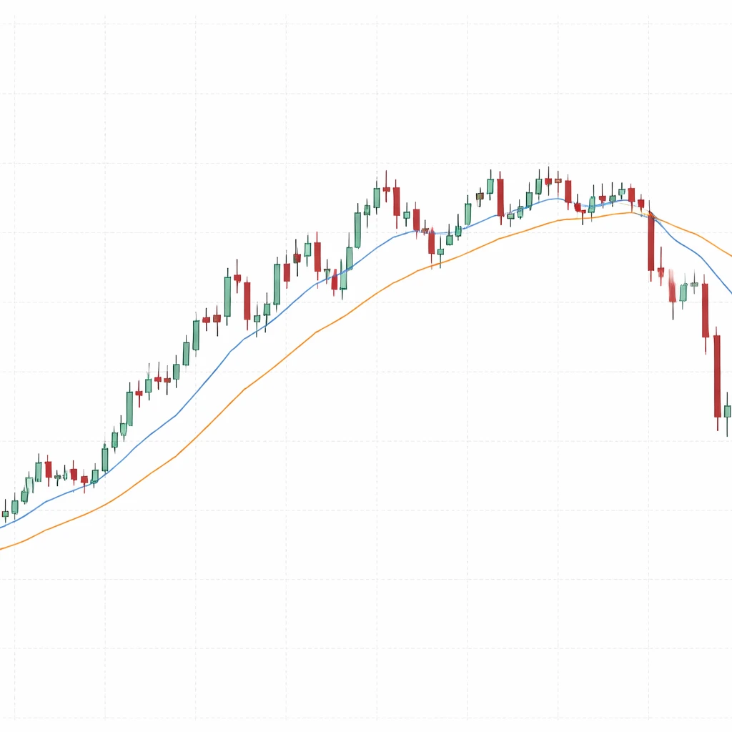
On a candlestick or bar chart, both SMA and EMA appear as smooth overlay lines tracking near price. Many charting packages default to distinct colors, such as a blue line for the SMA and an orange line for the EMA, with a small legend indicating length and type. The lines are continuous across the time axis and update at the close of each bar for close-based calculations.
When price is trending steadily, both lines will slope in the direction of the move. The EMA will often lie closer to price and bend sooner when the market turns. The SMA will lag slightly and display a smoother curve. In choppy or range-bound conditions, the EMA tends to weave closer to price, sometimes crossing above and below more frequently, while the SMA may remain flatter and further away from rapid fluctuations.
Weighting, Lag, and Responsiveness
Lag refers to the delay between a move in price and the response in the moving average. All smoothing introduces lag. Equal weighting across n observations dilutes the effect of the newest price to one part in n, which increases lag as n grows. The EMA reduces lag for a given n by placing greater weight on recent observations. The magnitude of this effect depends on the smoothing factor. For example, the 20-period EMA uses k = 2 ÷ 21, which weights the new price about 9.5 percent, whereas the 20-period SMA weights each of the 20 prices at 5 percent.
Responsiveness measures how quickly an average reacts to a new trend or to a shock. Because the EMA places more weight on recent data, it rotates more quickly when price direction shifts. The SMA changes direction only once enough new observations accumulate to outweigh the older values in the window. This is why in a sharp reversal the EMA will often turn before the SMA.
However, greater responsiveness also means the EMA will reflect more short-term noise. In markets where price flickers up and down around a central level, the EMA can oscillate around price more tightly and may produce more frequent crossings. The SMA, by distributing weight evenly, can be less sensitive to very short reversals and thus appear smoother.
Interpreting Price Relative to a Moving Average
Analysts often consider three aspects: the direction of the moving average, the position of price relative to the line, and the distance between price and the line. A rising line suggests that the average price over the chosen window is increasing. If price is consistently above the line, it indicates that recent prices have tended to exceed the past window’s mean. If the gap widens meaningfully, price may be moving away from its recent baseline at a faster rate, which can imply elevated momentum or stretched conditions depending on context.
The choice of SMA or EMA affects these interpretations. Because the EMA hugs price more tightly, the measured distance between price and the EMA is usually smaller than the distance between price and the SMA for the same n. As a result, the EMA can reattach more quickly after a sharp move, while the SMA may show a larger and more persistent gap until the window updates sufficiently.
Practical Examples in Chart Context
Consider a hypothetical equity that rises steadily from 100 to 120 over 30 sessions, with occasional two- or three-day pullbacks. Overlay a 20-period SMA and a 20-period EMA based on closing prices. As the equity advances, both lines slope upward. After a three-day pullback from 118 to 114, the EMA bends downward sooner and by a greater amount because the most recent closes carry more weight. The SMA flattens modestly but does not drop as quickly. When the price resumes upward movement, the EMA rotates upward first and closes the gap to price sooner, while the SMA follows with a delay.
Now consider a choppy period where price oscillates between 50 and 52 without clear direction. The 20-period EMA will track these small oscillations more closely, weaving slightly above and below price as it updates. The 20-period SMA will show a flatter profile and may lie closer to the midpoint of the range because equal weighting reduces the effect of the very latest bar. In this environment, the EMA may show more frequent interactions with price, whereas the SMA may appear steadier.
As a third example, imagine a news event that gaps price up from 60 to 66 at the open, followed by consolidation near 66. The 20-period EMA will jump toward the new level more quickly, due to the greater weight on the incoming price. The 20-period SMA will move up as well but will take several bars to converge toward the higher level, since much of its window still contains pre-gap values. This illustrates the general principle that the EMA adapts faster to abrupt changes, while the SMA preserves more of the prior price history.
Length and Timeframe Considerations
The lookback length n is as consequential as the choice between SMA and EMA. Shorter lengths capture recent changes quickly but with less smoothing. Longer lengths provide a more stable baseline but respond slowly. For any fixed n, the EMA will be the more responsive variant and the SMA the smoother variant.
Commonly referenced lengths include 10, 20, 50, 100, and 200 periods on daily charts, and analogous lengths on intraday or weekly charts. These values have become conventions rather than rules. Their relevance depends on the behavior of the asset and the analyst’s purpose. A 20-period line on a five-minute chart summarizes a different horizon than a 20-period line on a weekly chart. The arithmetic of the average remains the same, but the interpretation of stability or change must reflect the sampling interval of the data.
When comparing across timeframes, it is helpful to remember that the same lookback can imply different effective half-lives of information. For an EMA, the effective half-life is related to the smoothing factor and determines how quickly the influence of an old observation decays by half. On a faster timeframe with the same n, that half-life corresponds to a much shorter real-world duration.
Data and Calculation Details That Affect the Lines
Several implementation choices influence SMA and EMA values. Analysts should be aware of the following:
- Price input. Averages can be computed from closes, opens, highs, lows, typical price, or volume-weighted price. Close-based averages are most common, but using a different input changes the line’s level and shape.
- Session boundaries. Some intraday charts include pre- and post-market data. Others do not. Including additional sessions introduces more bars and can alter the average’s value at the regular open.
- Holiday and missing data. In markets with non-trading days, the number of calendar days differs from the number of sessions. Moving averages calculated by bars implicitly handle this, but gaps in data or incorrect timestamps can distort the series.
- Corporate actions and adjustments. For equities, split and dividend adjustments affect historical prices. A consistent back-adjusted series should be used so that the moving average reflects comparable values across time.
- Rounding and precision. Some platforms round intermediate values. Over many updates, rounding can introduce tiny differences between platforms, especially with EMAs due to the recursive formula.
Limitations and Common Misreadings
Moving averages are descriptive rather than predictive. They summarize what has occurred over a chosen window and therefore lag price by design. In a range-bound market, the line may appear to follow price back and forth without providing meaningful directional insight. In a volatile market with frequent reversals, a more responsive average will also reflect many short-lived moves. These are features of the smoothing process, not faults of a particular type.
Another common misreading is to treat small penetrations of the line as decisive information in isolation. Minor crosses can be artifacts of noise, particularly for shorter lengths or EMAs that emphasize the most recent bar. The frequency of such events depends on the volatility of the asset and the sampling timeframe.
Finally, there is a tendency to retroactively fit the length parameter to past price behavior. Selecting a lookback because it appears to align neatly with prior turning points in a single historical sample can overstate the usefulness of that parameter in other periods or on other assets. The observed fit may be coincidental and not robust.
Choosing Between SMA and EMA for Analytical Goals
The choice between SMA and EMA depends on what aspect of price behavior one wants to emphasize.
- Preserving historical context. If the purpose is to reflect the average level over a fixed window with equal representation of each observation, the SMA aligns with that goal. It makes each constituent bar contribute the same amount until it exits the window.
- Highlighting the latest information. If the goal is to adapt more quickly to recent changes and to reduce the footprint of older data, the EMA is suited to that purpose. It places larger weight on recent bars and decays older contributions smoothly rather than removing them abruptly at the window boundary.
- Visual aesthetics and interpretability. Some analysts prefer the smoother visual flow of the SMA for presentation or reporting. Others prefer the EMA’s faster curvature to illustrate developments in progress. These preferences reflect the type of narrative one wishes to draw from the data.
Crucially, both lines are valid representations of recent price, just with different weighting philosophies. The SMA treats all points in the window as equal. The EMA treats recent points as more informative. Understanding that distinction helps prevent over-interpretation of small differences between the two lines on a chart.
Relation to Smoothing and Filtering Concepts
From a signal processing perspective, a moving average is a linear filter. The SMA applies a rectangular window to the past n observations. This produces an impulse response that is finite in length and uniform in weight, and a frequency response that attenuates high-frequency fluctuations while preserving lower-frequency components. The EMA applies a decaying exponential kernel, which attenuates high-frequency components while introducing a different profile of phase delay and less abrupt truncation of the past.
These properties explain the observed chart behavior. The SMA, with its rectangular window, introduces a clear cutoff at the boundary of n periods. An old shock disappears all at once when it exits the window. The EMA never fully discards any observation, but reduces its influence continuously. As a result, the EMA tends to react earlier to new shocks and to let go of old shocks more gracefully.
Contextual Signals Without Strategy Prescriptions
Moving averages can be used to frame questions about price behavior without dictating specific trading actions. For example, observers often compare price to its average to judge whether a move is an extension relative to the recent norm. Others watch the slope of an average for a concise summary of directional drift over the lookback window. Some compare an SMA and an EMA of the same length to see how much the most recent action deviates from the broader mean. These contextual uses rely on the descriptive nature of the averages rather than on any prescriptive rule.
Putting the Concepts Together on a Chart
Suppose a daily chart of a liquid index displays both a 50-period SMA and a 50-period EMA. During a multi-week ascent, the EMA typically hugs the underside of price more closely on pullbacks, while the SMA runs modestly lower and smoother. When price stalls and transitions into a horizontal consolidation, the EMA flattens quickly and sits near the middle of the congestion range, while the SMA drifts toward flat with a slight delay. If a sudden downdraft occurs, the EMA bends down rapidly, and the SMA follows after several sessions as more declining closes enter the window.
This side-by-side view helps illustrate the practical differences. The EMA delivers a timelier reflection of new information. The SMA preserves a steadier reading of the recent average level. Neither is inherently superior. Each highlights a different aspect of the same underlying series.
Common Variations and Platform Settings
Most platforms allow customization. The following choices affect interpretation and comparability:
- Source price. Close, open, high, low, or combinations such as typical price. Changing the source alters the line.
- Offset or displacement. Some chartists display averages shifted forward or backward in time for visual spacing. This does not change the calculation but changes the visual alignment with price.
- Smoothing method labels. Labels like “EMA” may have minor implementation differences across vendors, especially for seeding and rounding. Documented details help reconcile small discrepancies between platforms.
When SMA and EMA Diverge Meaningfully
Although both lines often track closely, situations arise where the gap between them is informative about the recent pace of change. A widening gap suggests that recent prices differ materially from the older values in the window. For instance, after a sharp rise, the EMA may sit notably above the SMA for a while, reflecting the heavier weight on the new higher prices. In a prolonged sideways market, the two lines often converge and may be nearly indistinguishable because recent and older prices are similar.
The magnitude and duration of these divergences depend on volatility, the chosen length, and the intensity of recent moves. Observing this relationship can help frame the degree of recent acceleration or deceleration without implying any specific outcome.
Summary Perspective
Simple and Exponential Moving Averages share the same objective of smoothing price, yet they embody distinct weighting philosophies. The SMA is defined by equal weight within a fixed window, which produces a stable and relatively smooth line that changes almost mechanically as the window updates. The EMA is defined by exponential decay, which produces a line that responds faster to new information and reduces the influence of older data gradually. On a chart, these differences manifest as slight contrasts in curvature, alignment with price, and speed of rotation during transitions. Understanding these mechanics equips analysts to interpret the lines as descriptive tools that place current price movements in recent historical context.
Key Takeaways
- The SMA assigns equal weight to the last n prices, while the EMA weights recent prices more heavily via exponential decay.
- For the same length, the EMA reacts faster to new information and typically hugs price more closely than the SMA.
- Both lines are lagging summaries of past prices, so differences between them reflect weighting choices rather than predictive power.
- Chart context matters: in sharp moves the EMA turns earlier, while in quiet ranges the SMA may appear smoother and more stable.
- Calculation inputs, data handling, and length selection materially affect the look and interpretation of both averages.