Moving averages are among the most widely used tools in technical analysis. They transform a series of prices into a smoother line that represents the average of recent observations. The appeal is straightforward. Prices can be volatile from one period to the next, and a moving average reduces that variability to reveal a clearer view of the prevailing direction and the market’s central tendency over a chosen window.
This article explains what a moving average is, how different variants are constructed, and how they appear on charts. It also examines why these lines often attract attention in market commentary. Throughout, the focus remains on interpretation of price behavior rather than on strategies or recommendations.
What is a Moving Average?
A moving average is a rolling statistic computed over the most recent N observations. In price analysis, the observations are typically closing prices at a fixed sampling interval such as daily, hourly, or 1-minute bars. As each new bar completes, the average incorporates the new price and discards the oldest one inside the window. The result is a series of averaged values that changes more slowly than raw price, which makes broad direction easier to see.
Three main properties define any moving average:
- Input price: close is common, but some analysts use typical price (high + low + close divided by 3), median price (high + low divided by 2), or other transformations.
- Window length: the number of observations N used in the average. Larger N produces more smoothing and more lag. Smaller N produces less smoothing and less lag.
- Weighting scheme: how much influence each observation within the window has on the computed average. Simple moving averages apply equal weights. Exponential averages apply heavier weights to recent observations. Other schemes exist as well.
How Moving Averages Appear on Charts
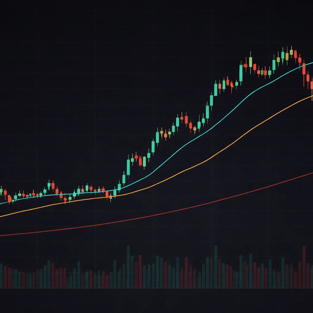
On a price chart, a moving average is drawn as a continuous overlay line that follows price but with reduced volatility. If you overlay a short window such as a 10-period average and a longer window such as a 100-period average, the short line will hug price more tightly while the long line will be smoother and slower to react. Many charting platforms show the average as a colored line plotted on top of candlesticks or bars, often accompanied by additional averages in different colors for visual comparison.
Common conventions include:
- Short windows such as 5 to 20 periods to observe near-term direction and momentum.
- Intermediate windows such as 50 periods to characterize multi-week or multi-month trends on daily charts.
- Long windows such as 100 or 200 periods to capture broad trends across seasons or cycles.
The exact values vary by market, timeframe, and analytical preference. What matters is understanding the trade-off between smoothness and responsiveness, since that trade-off shapes how the line behaves relative to the underlying price series.
Why Analysts Watch Moving Averages
Moving averages serve as descriptive statistics that help interpret price behavior. They are not predictive in a strict sense. Their value lies in what they summarize.
- Noise reduction: Averages filter out a portion of short-term variability and make slow-moving changes in direction more apparent.
- Central tendency reference: The average acts as a dynamic benchmark. The distance between price and the average provides a sense of how stretched or compressed price is relative to its recent history.
- Temporal context: Different windows frame price action across multiple horizons, which can clarify whether shorter-term movements align with or diverge from longer-term direction.
- Comparability: Averages standardize observation. Two analysts can discuss the same 50-period average and refer to an identical calculation rather than a subjective impression of the chart.
Common Types of Moving Averages
Simple Moving Average
The simple moving average, or SMA, is the arithmetic mean of the last N prices. If P denotes the closing price, the 5-period SMA at time t equals the average of P at t, t-1, t-2, t-3, and t-4. Each observation contributes equally to the result.
Properties of the SMA include strong smoothing for larger N and a lag equal to roughly half the window length. For example, a 20-period SMA responds to a change in price with an average delay of about 10 periods because it incorporates the last 20 values equally.
Exponential Moving Average
The exponential moving average, or EMA, assigns more weight to recent prices. It is computed recursively: EMA at time t equals EMA at time t-1 plus alpha times the difference between price at t and EMA at t-1. The smoothing constant alpha is commonly set to 2 divided by (N + 1), where N is the chosen span. This formulation maintains the intuitive mapping between EMA length and responsiveness.
Compared with the SMA at the same N, the EMA reacts faster to recent changes and therefore exhibits less lag while offering slightly less smoothing. Its effective weighting decays exponentially across past observations rather than cutting off abruptly at N.
Weighted Moving Average
The weighted moving average, or WMA, applies linearly decreasing weights from the most recent observation back to the Nth observation. For example, with N equal to 5, the most recent price might receive weight 5, the prior price weight 4, and so on down to weight 1. This design lies between the SMA and EMA in concept. It rewards recency but with a finite window and a linear, not exponential, decay.
Volume-Weighted Moving Average
The volume-weighted moving average, or VWMA, incorporates trading volume into the weights. Observations with higher volume influence the average more than low-volume observations. The VWMA can be useful for analysts who wish to emphasize prices that occurred with greater participation. The trade-off is that the line may respond differently during low-liquidity periods, which can complicate comparisons with price-only averages.
Other Variants
Triangular, smoothed, Hull, and adaptive moving averages are also used. Each tries to balance smoothness and lag in a particular way. The core interpretive ideas remain the same. A longer effective window yields more smoothing and more delay. A heavier emphasis on recent prices reduces lag but can reintroduce noise.
How Moving Averages Are Constructed
Construction begins with selecting a price input, a sampling interval, and a length. A typical setup uses daily closing prices and a length such as 20, 50, or 200 periods. The SMA computes the arithmetic mean over the last N closes. The EMA uses the recursive update described above with alpha equal to 2 divided by (N + 1). The WMA applies a chosen weight schedule that sums to 1. The VWMA multiplies each price by its volume, sums across the window, and divides by total volume in the window.
Several practical details matter in implementation:
- Warm-up period: An EMA requires a seed value to start. Many charting systems initialize the first EMA to the first available price or to an SMA of the first few periods. The earliest values can be less reliable because the average has had little history to stabilize.
- Data adjustments: For equities, adjusted closes account for splits and dividends. Using adjusted prices yields a more coherent series across corporate actions and tends to produce moving averages that align more meaningfully with historical price paths.
- Holidays and illiquid periods: On markets with irregular trading days, the count of periods still advances only when a bar exists. The meaning of a 200-day average reflects 200 trading days, not calendar days.
- Intraday noise: Short intraday windows on fast timeframes can respond to microstructure effects such as bid-ask dynamics. Longer windows reduce these effects at the cost of additional lag.
Smoothing, Lag, and the Signal-to-Noise Trade-off
The benefit of smoothing is easiest to see at turning points. A short window often changes direction quickly, while a long window changes direction only after sustained movement. This behavior can be described in terms of lag. For an N-period SMA, average lag is approximately N minus 1 over 2 periods. An EMA with span N has a somewhat smaller effective lag that depends on alpha. The general idea holds that more smoothing implies more delay in the average reflecting a new trend.
From a signal processing perspective, a moving average acts as a low-pass filter. It attenuates high-frequency fluctuations and passes lower-frequency movements. The SMA, with its flat weights and sharp cutoff at N, can introduce oscillations in the presence of abrupt price changes. The EMA’s exponential decay produces a smoother response to shocks. This perspective explains why two moving averages with the same N can behave differently in volatile conditions.
Interpreting Moving Averages on Charts
Moving averages translate into several visual cues that analysts use to describe price behavior:
- Slope and curvature: The slope of the average indicates whether the recent mean is rising or falling. A flattening slope suggests deceleration. A re-accelerating slope suggests renewed directional movement.
- Relative position: The location of price relative to its average characterizes whether price is above or below its recent central tendency. The vertical distance between price and the average can be expressed in points, as a percentage, or in standard deviations if one also computes volatility.
- Multiple averages: Overlaying short, intermediate, and long averages provides a layered view of different horizons. Alignment or dispersion among these lines conveys how short-horizon action compares with longer-horizon direction.
- Behavior around the line: In some markets, price appears to gravitate toward the average after extended deviation. In others, price may overshoot and oscillate around it. These tendencies can vary across assets and regimes.
Practical Chart-Based Context
Consider a daily chart of a hypothetical company, XYZ Corp, spanning January to December. Overlay a 20-day EMA and a 100-day SMA. Early in the year, suppose price rallies sharply for several weeks. The 20-day EMA responds quickly, turning upward within a few days and tracking close to the candles. The 100-day SMA turns up only after the rally persists long enough to influence the majority of its window. If price then consolidates sideways for a month, the 20-day EMA tends to flatten and weave near price, while the 100-day SMA continues to drift gently higher because it still reflects the earlier advance.
Later in the year, imagine a sharp one-week decline. The 20-day EMA bends down promptly, while the 100-day SMA softens only slightly. If price rebounds within a few sessions to its prior range, the 20-day EMA pivots again, highlighting how a short EMA is sensitive to rapid changes. The 100-day SMA remains comparatively steady, which clarifies the longer-term average context despite short-term turbulence.
This side-by-side visualization is instructive. It shows that a short average is better at showing immediate shifts, and a long average is better at showing the broad trend. Neither is right or wrong. They serve different descriptive roles, and the analyst chooses the horizon that matches the question at hand.
Distance from the Average
The difference between price and its moving average is a useful descriptive quantity. It can be measured as price minus average in currency units, as a percentage of the average, or standardized by volatility. Large positive distances indicate price is extended above its recent mean. Large negative distances indicate price is extended below it. The size and persistence of these distances tend to vary by asset class and volatility regime. For example, a high-volatility equity index may see frequent double-digit percentage gaps relative to a 20-day average, while a low-volatility bond future may show much smaller relative deviations.
An analyst might also examine how distance evolves through time. If price oscillates around the average with contracting amplitude, it suggests consolidation. If distances expand and stay one-sided, it suggests directional persistence. These observations remain descriptive and do not imply any particular decision.
Multiple Averages for Context
Using more than one moving average on the same chart can provide context across horizons. A common illustration is to place a short average such as a 20-day EMA, an intermediate average such as a 50-day SMA, and a long average such as a 200-day SMA. When the short average spends time above the long average, it indicates that recent prices are, on average, higher than the longer-term mean. When the short average is below, the opposite holds. The distances among the averages communicate the degree of alignment or dispersion across timeframes.
Crossings of one average over another show changes in the relationship between recent and longer-term means. Analysts often reference these crossings in commentary because they are easy to identify and communicate. The crossing itself, however, is still a consequence of the chosen windows and weights, not a natural boundary in the market.
Window Selection and Interpretation
Selecting a window length involves a clear trade-off. Short windows deliver responsiveness and detail but are prone to whipsaw in volatile ranges. Long windows deliver steadiness but reflect changes with delay. The best choice depends on the timeframe under study and the purpose of the analysis. For example, a researcher interested in monthly trends might consider a 6-month or 12-month average on monthly data, while an intraday analyst might look at a 30-minute average on 1-minute bars. Each choice frames the data differently and will lead to different visual conclusions about trend and deviation.
It is also essential to keep the sampling interval in mind. A 50-period average on 1-minute bars covers 50 minutes of trading, while a 50-period average on daily bars covers approximately ten weeks of trading days. The numerical length is the same, but the economic meaning is not.
Moving Averages and Oscillators
Moving averages are trend-following indicators, not oscillators. They do not inherently fluctuate around a fixed center unless price is stationary around a constant level. However, analysts often construct oscillators derived from moving averages. Two common examples are:
- Price minus moving average: an oscillator that measures distance from the mean and shows over or under extension relative to the chosen horizon.
- Moving average convergence and divergence concepts: differences between short and long moving averages form the basis of indicators that oscillate around zero, highlighting shifts in relative momentum without requiring a directional threshold.
These derivatives of moving averages serve different interpretive needs. The moving average itself provides the baseline, while the oscillator quantifies deviation or rate of change around that baseline.
Data Choices and Their Consequences
The choice of input price can shape the appearance of a moving average, especially for short windows. Using typical price or median price can reduce the influence of outlier closing prints on illiquid bars. Some analysts prefer the average of high, low, and close to integrate intrabar information. Volume-weighted versions place more emphasis on periods with higher participation, which can be informative in markets where volume varies widely through the session or across days.
For equities, adjusted closing prices that account for splits and dividends are often preferable for historical analysis. Without adjustment, a large dividend can create an artificial gap that depresses the average even though the economic value did not change in the same way. Adjusted data presents a continuous series that aligns more closely with investor total return.
Interpreting Behavior Around the Average
Many observers note that price sometimes pauses near a widely followed moving average. Whether this reflects self-reinforcing attention, underlying market structure, or randomness varies by context. What can be said with confidence is that the moving average represents a level of central tendency. When price has wandered far from that center, a return toward it is a common pattern in many markets. When price has remained close to the average, a sudden expansion away from it can signal a regime shift in volatility or participation. These interpretations remain descriptive rather than prescriptive.
Gaps, Regime Changes, and Structural Shifts
Because moving averages are backward looking, they summarize the past. A structural change in the market, such as a macroeconomic shock or a company-specific development, can cause price to gap far from the existing average. The average will follow only gradually. During such periods, the lag is visible, and the average can sit well behind fast-moving price. Observing the rate at which the average catches up can be informative about the persistence and magnitude of the change.
Limitations and Common Pitfalls
- Whipsaw in ranges: In sideways markets, short moving averages often change direction frequently. The frequent reversals reflect noise more than new information about trend.
- Parameter sensitivity: Small changes in window length or weighting can alter signals and historical interpretations. This sensitivity increases the risk of overfitting when one searches for a length that best fits past data.
- Look-ahead bias: Moving averages must be computed only with information available at each point in time. Using the full dataset to refine parameters and then measuring historical performance can produce misleading impressions of robustness.
- Data quality: Missing bars, stale quotes, or unadjusted corporate actions can distort the average and its relationship to price.
- Uniformity across assets: A 50-period average may behave very differently across assets with different volatility profiles and trading hours. Comparisons require care.
Worked Visual Example
Imagine a chart of a liquid equity index over two years. Overlay a 50-day SMA and a 200-day SMA. During a prolonged advance, the 50-day SMA stays above the 200-day SMA and maintains a positive slope. When the index enters a multi-month consolidation, the 50-day SMA flattens and can weave closer to the 200-day SMA. If a deep correction occurs, the 50-day SMA may descend toward the 200-day SMA. During the recovery that follows, the 50-day SMA responds first while the 200-day SMA changes direction later. No single moment on this chart tells a complete story. The value comes from seeing how the averages summarize the prevailing trend at different horizons and how price behaves around these slow-moving references.
Intraday Considerations
On intraday charts, moving averages can be influenced by market microstructure. Opening auctions, lunch-hour lulls, and closing rotations can concentrate volume and price movement into specific segments of the day. A VWMA will emphasize these segments more than an SMA or EMA. Very short windows on 1-minute data can track noise rather than meaningful shifts in supply and demand. Longer intraday windows, such as a 60-minute average on 5-minute bars, produce a smoother path that dampens microstructure effects.
Combining With Volatility Measures
Because moving averages capture central tendency, pairing them with a dispersion measure can be useful for context. One simple approach is to compute the standard deviation of price over the same window and express the distance between price and the moving average in standard deviations. Large absolute values indicate that price is far from its recent mean relative to typical variation. This pairing helps distinguish between a small nominal distance that is large in standardized terms and a large nominal distance that is modest in a high-volatility regime.
Interpreting Slopes and Inflection Points
Slopes and inflections carry information about the rate of change in the average itself. A rising slope indicates that recent prices, on average, exceed the values from earlier in the window. The point at which a previously rising average begins to flatten indicates that the recent sequence is no longer consistently higher than the earlier sequence. An inflection back upward indicates a renewed sequence of higher recent values. This logic holds across SMA, EMA, and WMA, though the timing differs because of the weighting scheme.
Context Across Markets
In equity indices, market participants often reference very long averages such as the 200-day SMA because they help frame multi-quarter direction. In commodity futures, where seasonality and roll mechanics can influence the series, analysts often choose windows that reflect cycle length or delivery patterns. In foreign exchange, where trading is continuous across global sessions, intraday windows that capture major session overlaps can be informative. The core principle remains to select windows whose economic meaning aligns with the behavior under study.
Implementation Notes for Researchers
- Rolling computation: Efficient implementations maintain running sums for SMAs and recursive updates for EMAs. This matters for high-frequency or long-history datasets.
- Missing values: Define a consistent rule for handling missing bars. Dropping them is common, but interpolation can distort the meaning of the average.
- Anchoring: Some studies use anchored or cumulative averages that start from a fixed date. These differ from rolling averages and have different interpretive properties.
- Outliers: Filters that cap extreme moves can stabilize short-window averages in datasets with occasional bad prints. Care is needed to avoid removing legitimate market moves.
What Moving Averages Do Not Do
A moving average does not forecast turning points on its own. It does not identify intrinsic value. It does not adjust to new information except through the lens of its chosen window and weights. It is a descriptive overlay that summarizes where price has been and how that history distributes across recent periods. When analysts discuss interactions with moving averages, they are describing relationships in the data rather than asserting predictive rules.
Putting It All Together
Moving averages distill complex price action into a stable reference. By selecting a specific window and weighting scheme, an analyst chooses the horizon and responsiveness of the summary. The resulting line helps contextualize current price, clarifies direction at the chosen timescale, and organizes the chart into interpretable patterns of trend and deviation. Used thoughtfully, moving averages improve clarity without imposing a rigid narrative on every fluctuation.
Key Takeaways
- Moving averages are rolling summaries of recent prices that reduce noise and highlight central tendency at a chosen horizon.
- Different weighting schemes, such as SMA, EMA, WMA, and VWMA, trade off smoothness and lag in distinct ways.
- The slope of the average and the distance between price and the average provide descriptive context about direction and extension.
- Multiple averages on the same chart organize information across short, intermediate, and long horizons without implying specific actions.
- Choice of window length, input price, and data adjustments materially affects how a moving average behaves and how it should be interpreted.